What is SVM?
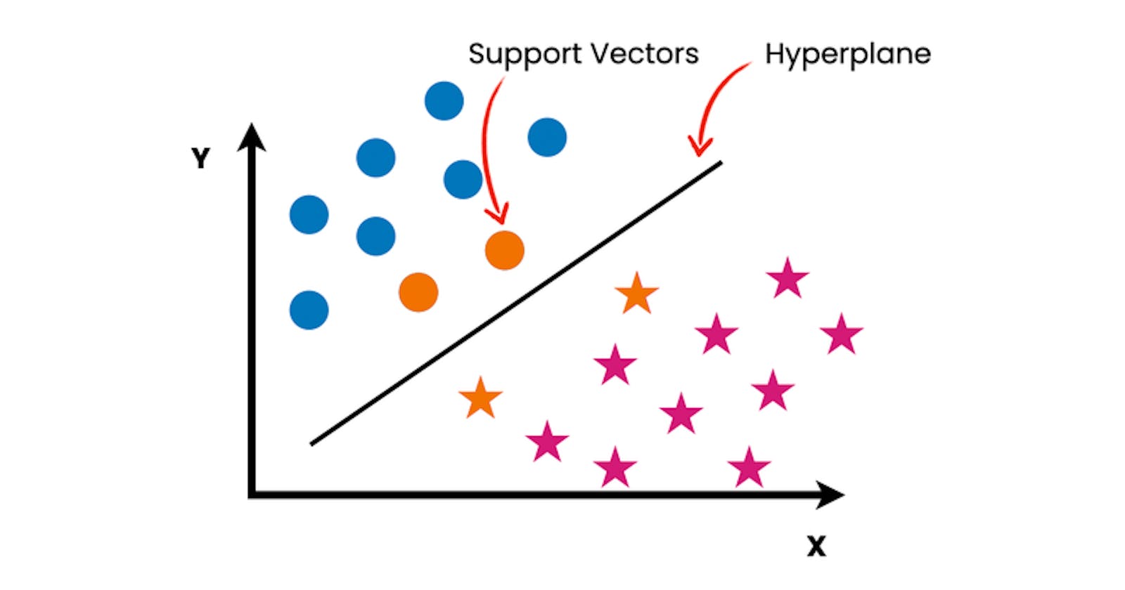
Support Vector Machine is a supervised machine learning algorithm. It is mostly used for classification problems. The objective of SVM algorithm is to find a hyperplane (more about it later in the article) that will distinctly classify the data points. Support vector machine is highly preferred by many as it produces significant accuracy with less computation power.
Maximal Margin and Support Vector Classifier
Suppose we have a dataset with only 1 feature like mass in the below example -

The shortest distance between the threshold (vertical bold line) and the nearest observation of opposite labels is called margin.
At the exact center of the distance between the observation of opposite labels, the margin is maximum. This margin is called Maximal Margin Classifier.
Maximal Margin Classifier is not useful because it will give bad predictions if our dataset have outliners like this -

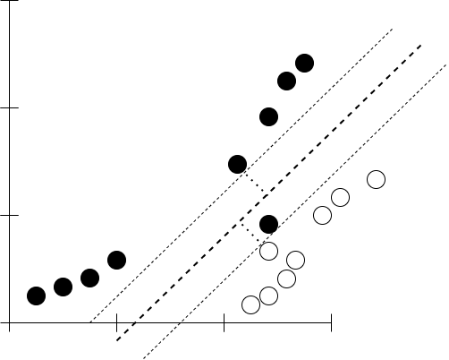
In this case, we must allow some misclassifications to determine the optimal location of our threshold line. When we allow misclassifications, the distance between the observations and the threshold is then called a Soft Margin. Soft Margin is determined with the help of cross validation and bias/variance tradeoff. Classification done with the help of soft margin is called Soft Margin Classifier aka Support Vector Classifier. The observations at the edge and within the soft margin are called Support Vectors.

In the diagram above, observations from 5 to 9 are called support vectors.
Support Vector Classifier for a 2 dimensional dataset would like this -

In this case, the support vector classifier is a line. When dataset is of 3 dimension, we would have a plane as support vector classifier. For higher dimensions and also for these 3 dimensions, the support vector classifier is called a hyperplane.
Suppose we have a dataset like below -

In this case, drawing a threshold anywhere on the graph will give a lot of misclassifications. So, support vector classifier doesn't work with all types of dataset. Here comes the Support Vector Machine.
SVM Algorithm
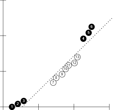
SVM algorithm transforms the data from current dimension to higher dimension using a kernel function. The above example can be transformed by squaring the values and then we find the support vector classifier on this new transformed data.

Kernel Functions
Polynomial Kernel Function
In the above example, I used the Polynomial Kernel which has a parameter d that stands for degree of the polynomial. After plugging the value of d to the algorithm, the relationships between each pair of transformed observations are used to find a support vector classifier. We can find the optimal value of d using cross validation. One important thing to note here is the kernel function only calculates the relationships between every pair of points as if they are in the higher dimensions, it does not actually do the transformation. This is called the kernel trick. The kernel trick saves us a lot of computation power by avoiding the math required for transforming data. The equation of polynomial kernel looks like this -

a and b refers to two different observations in the dataset.
r is the coefficient of polynomial.
d is the degree of the polynomial.
We plug the values and get high dimensional relationship between the observations.
Radial Kernel Function
It is also known as Radial Basis Function (RBF). The equation of RBF looks like -

Radial Kernel Function behaves like a weighted nearest neighbor model. In other words, the closest observations have a lot of influence on how we classify and observation that are far away have relatively little influence on the classification. Mathematically we can prove that Radial Kernel finds Support Vector Classifier in infinite dimensions so it is impossible to visualize it.
Conclusion
In this article we learned what are margins, hyperplanes, how support vector machine solves different classification problem and two types of kernels - polynomial and radial.
