Introduction

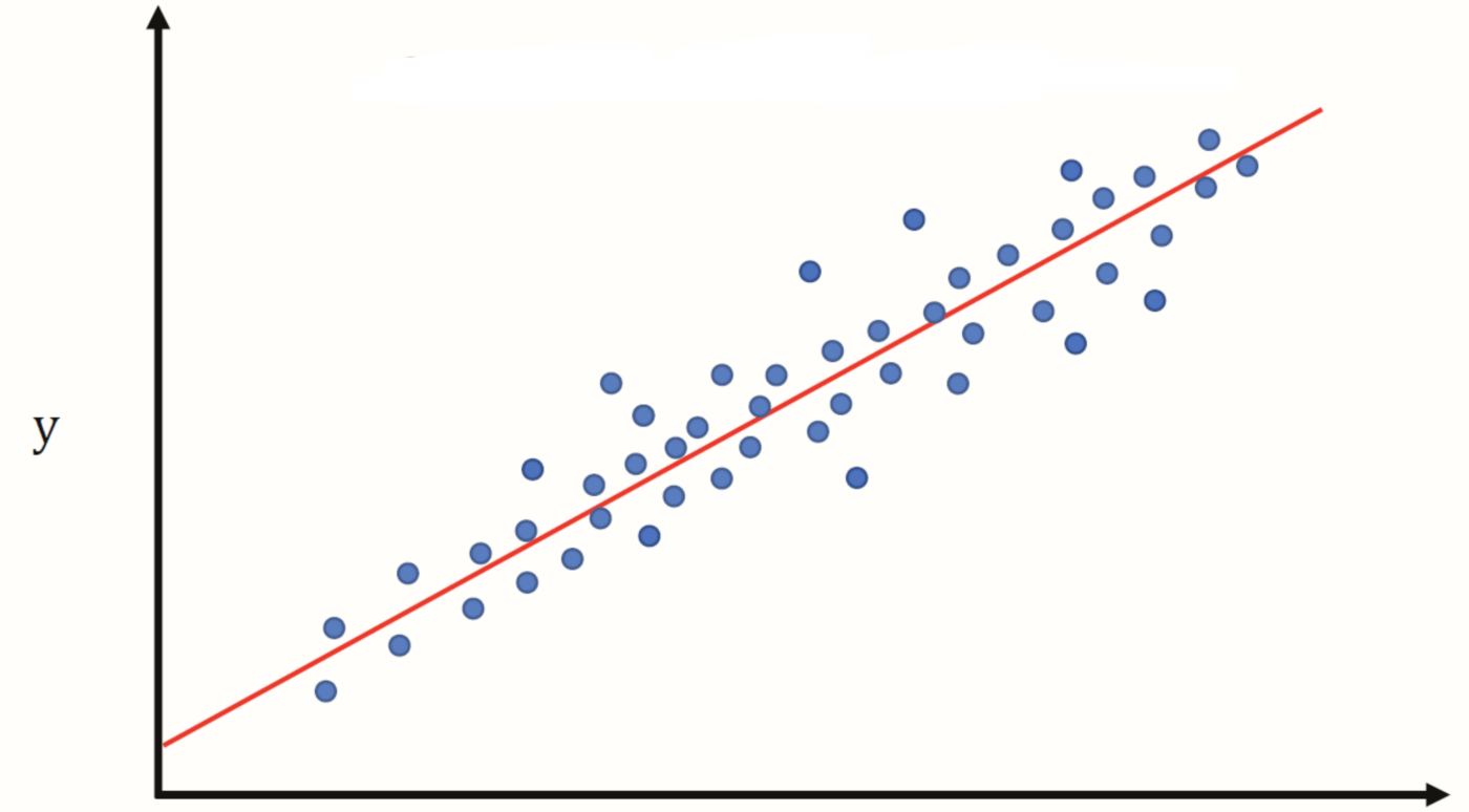
Linear Regression is a supervised machine learning model used to predict a quantity (continuous values) such as price of a stock, car prices, temperature of a place, etc. The model tries to find the best fit linear relationship between the target value and one or more predictor (input value). In this article, I will try to explain how Linear Regression model works.

Hypothesis

Linear Regression model tries to map the linear relationship between the input and output using the following equation -

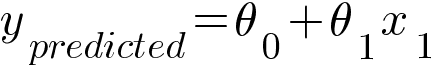In the equation, θ₀ is the y-intercept and θ₁ is the slope of the line.

In case of multiple inputs which we call it as Multiple Linear Regression, the hypothesis will look like this -

The model tries to predict the values of θ which will produce the best fit linear line. This is carried out using loss function and optimizer discussed further in the article.

Loss function

Loss function also known as the cost function tells us the error between the predicted value and the actual value. Root Mean Squared Error (RMSE) is the most used loss function in Linear Regression Model.

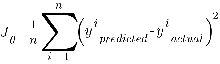
n in the equation is the number of observations, y_predicted is the predicted value generated using the hypothesis function and y_actual is the actual value. Our goal is to minimize this loss function which is achieved using an optimizer.

Optimizer

To update θ₀ and θ₁ values in order to reduce RMSE value and achieve the best fit line, the model uses an optimizer. There are many optimizers but the most famous of them is Gradient Descent Algorithm. The idea behind gradient descent algorithm is we first start with a random value of θ₀ and θ₁ mostly 0 and iteratively update the values using some formulae. The formulae are as follows -

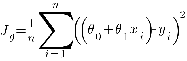
Substituting hypothesis equation in RMSE we get -

Calculating partial derivative of θ₀ and θ₁ with respect to the above RMSE equation.

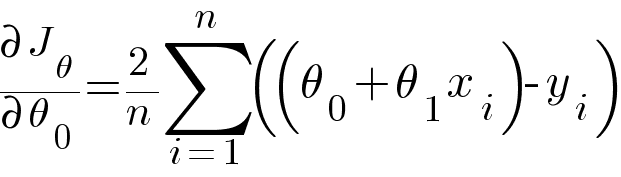
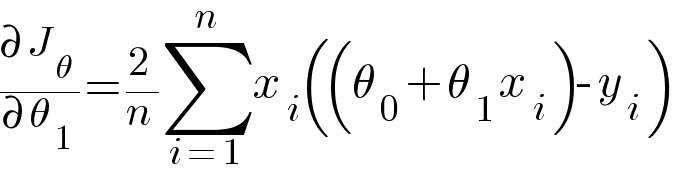
Then updating the values of θ₀ and θ₁ using the following equation -

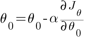
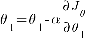
In the above equations, α is the learning rate which is a predetermined constant. The ideal value of α is between 0.01 to 0.001.

We iteratively run the above equations for 1000 to 10000 times to find the perfect values of θ₀ and θ₁ and achieve minimum cost function.

The python code for gradient descent algorithm -

import numpy as np

def gradient_descent(x,y):
    theta1_curr = theta0_curr = 0
    iterations = 10000
    n = len(x)
    learning_rate = 0.08

    for i in range(iterations):
        y_predicted = theta0_curr + theta1_curr * x

        loss = (1/n)*sum([val**2 for val in (y_predicted - y)])

        theta0_partial = (2/n)*sum(y_predicted - y)
        theta1_partial = (2/n)*sum(x*(y_predicted - y))

        theta1_curr = theta1_curr - learning_rate * theta1_partial
        theta0_curr = theta0_curr - learning_rate * theta0_partial

        print ("m {}, b {}, loss {} iteration {}".format(theta1_curr, theta0_curr, loss, i))

x = np.array([1,2,3,4,5])
y = np.array([5,7,9,11,13])

gradient_descent(x,y)

Code

We can directly use the LinearRegression module from the scikit-learn library. By doing so, we just have to abstract the module and the library will take care of its implementation.

import numpy as np

# data
x_values = [i for i in range(11)]
y_values = [i * 2 + 1 for i in x_values]

X = np.array(x_values, dtype=np.float32).reshape(-1, 1)
y = np.array(y_values, dtype=np.float32).reshape(-1, 1)

from sklearn.linear_model import LinearRegression
from sklearn.model_selection import train_test_split

X_train, X_test, y_train, y_test = train_test_split(X, y, test_size=0.20, random_state=0)

model = LinearRegression()
model.fit(X_train, y_train) # training the model

print(model.intercept_) # value of theta_0
print(model.coef_) # value of theta_1

y_pred = model.predict(X_test) # predicting value

print(y_test)
print(y_pred)

Conclusion

In this article we learned how Linear Regression works. It is best to not go too much into the math behind any model because almost all the time we will be using libraries which have already implemented the models for us.